Oversampled Peak Detection

Q: How does oversampled peak detection work?

Oversampling is sometimes used in order to improve the accuracy of peak level estimates for sampled signals. The idea is that when a signal is sampled, there may be no samples taken at or near the peak values of the signal. When this happens, the maximum sample-values will not be equal (or close) to the peak values of the signal. Oversampling increases the density of samples, with the hope that some of the (newly calculated) additional samples will be near the peaks of the signal. These additional sample values can be used to make an improved estimate of the peak signal level.

Our ability to oversample a signal depends on the sampling theorem, which states that as long as a signal is band limited to one half the sampling rate, the signal can be reconstructed from its samples. In other words, a collection of samples uniquely defines a continuous-time, band limited signal. Values of the signal can be calculated for any points in time based solely on that signal’s sample values. The oversampling process can be thought of as interpolation; the signal is reconstructed at discrete points in time which lie between the existing samples.

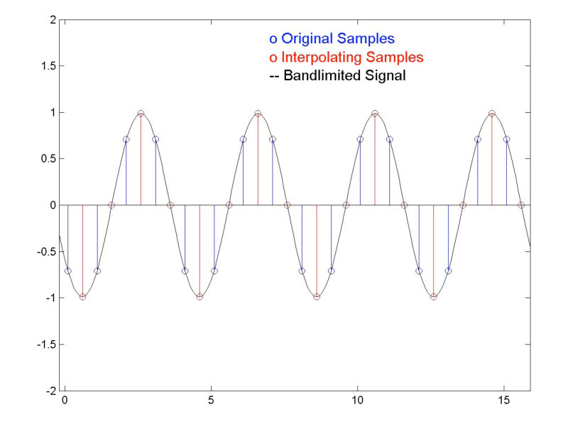
Figure 1 shows a continuous-time sine wave that has been sampled, and then subsequently oversampled by a factor of two. The original samples are shown in blue, with the oversampled points in red. As can be seen, none of the blue samples approach the peak value of the sine wave. However, some of the red points fall directly on the peaks of the wave. For this signal phase, oversampling reduces the peak estimate error from 3 dB (the value of the blue samples) to 0 dB.

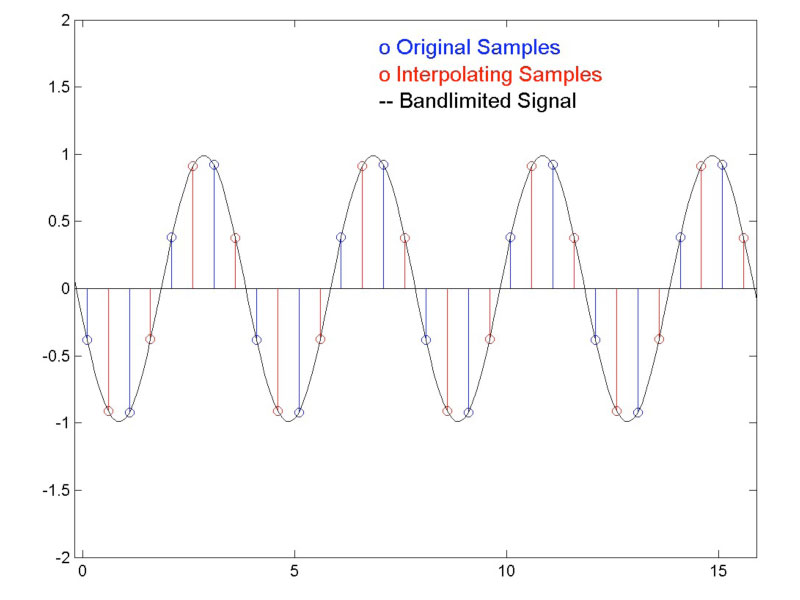
If we happen to sample the same signal at a different phase, as in Figure 2, we get a smaller error for the original samples (0.6877 dB), but oversampling by a factor of two does not change the peak estimate error: The red samples fall at the same values as the blue samples.

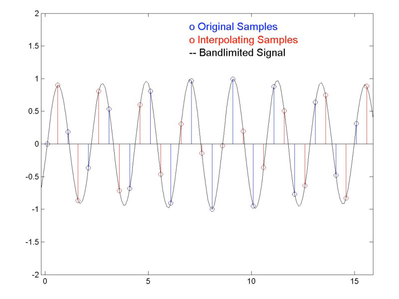
Usually, the sampling rate will not be an exact multiple of the signal frequency. If that is the case, we get a sampled signal as shown Figure 3. Here, the original samples may approximate the signal peaks closely in some areas, and in other areas not so closely. This can lead to a peak estimate that fluctuates over time. It can be seen from the figure that oversampling (taking the red and blue samples together) can reduce the variation over time of the peak estimate.

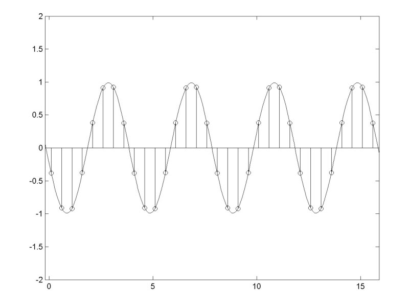
The worst-case peak-detection error for a sinusoid is shown in Figure 4, where the sampling rate is a multiple of the signal frequency, and the samples are evenly spaced around the signal peaks. For this case, the error in dB is equal to -20*log10(cos(πf0/fs)), where f0 is the frequency of the input, and fs is the sampling rate. The error is largest for an input frequency of fs/2, and takes on the value -20*log10(cos(π/2Ν)) for an oversampling factor N, assuming “perfect” oversampling. Maximum errors for some different oversampling rates are shown in the table below.

The most common rationale given for oversampled peak detection is that peak signal values must be known in order to prevent distortion during signal playback. The argument is that D/A converters have a finite amount of headroom: If the continuous signal has peaks at levels substantially higher than the largest recorded sample, the D/A converters will saturate, creating distortion. The above table is commonly used as a guideline to determine how much additional headroom will be needed for a D/A converter, given a particular oversampling rate. Conversely, the table could be used to build in a safety factor when producing digitized recordings. For a given oversampling factor, if the largest samples are constrained to be below the maximum allowed level by the amounts shown in the table, some argue that the continuous signal will be bounded by the maximum possible sample level, allowing for distortion-free playback of the signal.

The problem with the method as outlined above is that the safety margins given are only valid for sinusoidal signals. For non-stationary signals, the margins are inadequate. In fact, for arbitrary-length signals, the difference between oversampled peak estimates and actual peak levels can’t be bounded. Consider the pathological case:

x(n) = -(-1)n n>0
x(0) = 1
x(n) = -x(-n) n<0

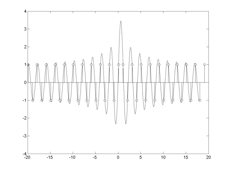
As shown in Figure 5, this signal alternates between +1 and -1, with two consecutive +1 samples at n=0,1. The interpolated peak signal value at the location n=0.5 grows logarithmically with the length of x, so that if x is infinitely long, the peak value is also infinite. For a signal x, which would barely fit on an audio CD, the peak signal value is about 22dB above the largest sample value! The situation is further complicated by the fact that the calculated oversampled peak value depends on the length of window used in the oversampling filter.

Figure 5 shows the calculated interpolated signal for an oversampler with a length of 32. This gives an interpolated peak about 11dB above the largest sample value. The calculated peak value grows logarithmically with the length of oversampling window used.

One possible alternative method to choose levels for digitally encoded signals would be to oversample by a high factor using an interpolation filter that simulates the behavior of a typical D/A reconstruction filter. Such an approach would not estimate the “ideal” peak signal levels; rather, it would create an estimate of the headroom needed for D/A conversion. In any event, it is clear that care should be taken when dealing with digitally encoded signals, as peak signal levels can fall significantly above maximum sample values.

— Dr. Dave Berners